Difference between revisions of "Lorenz"
| (4 intermediate revisions by the same user not shown) | |||
| Line 1: | Line 1: | ||
In 1963 Edward Norton Lorenz (23.05.1917 - 16.04.2008) developed a model for atmospheric convection (see https://journals.ametsoc.org/view/journals/atsc/20/2/1520-0469_1963_020_0130_dnf_2_0_co_2.xml and https://www.math.uni-hamburg.de/home/lauterbach/scripts/seminar03/prill.pdf for more details). This model, which was simulated on a tiny digital computer (Royal McBee LPG-30), showed an interesting behaviour which gave rise to research on chaotic attractors. | In 1963 Edward Norton Lorenz (23.05.1917 - 16.04.2008) developed a model for atmospheric convection (see https://journals.ametsoc.org/view/journals/atsc/20/2/1520-0469_1963_020_0130_dnf_2_0_co_2.xml and https://www.math.uni-hamburg.de/home/lauterbach/scripts/seminar03/prill.pdf for more details). This model, which was simulated on a tiny digital computer (Royal McBee LPG-30), showed an interesting behaviour which gave rise to research on chaotic attractors. | ||
| − | The system itself is described by three | + | The system itself is described by three coupled differential equations (x' denotes the first derivative of x with respect to time here - more typically it would be written with a dot over the variable name): |
x'=σ(y-x)<br> | x'=σ(y-x)<br> | ||
| Line 7: | Line 7: | ||
z'=xy-βz<br> | z'=xy-βz<br> | ||
| − | In the original system the parameters are σ=10, β=8/3, and ρ=28. Obviously, this cannot be implemented on an analog computer directly as it is not scaled to the interval [-1,1]. Scaling this system is a bit cumbersome: First, the domains of all involved variables have to be determined. Scaling and rewriting the system yields the following set of equations: | + | In the original system the parameters are σ=10 (that is the Prandtl number), β=8/3 (this represents the cell geometry underlying the model), and ρ=28 (relative Rayleigh number). Obviously, this cannot be implemented on an analog computer directly as it is not scaled to the interval [-1,1]. Scaling this system is a bit cumbersome: First, the domains of all involved variables have to be determined. Scaling and rewriting the system yields the following set of equations: |
x=∫1.8y-x dt+C<br> | x=∫1.8y-x dt+C<br> | ||
| Line 30: | Line 30: | ||
[[File:lorenz_THAT_setup.jpg|768px]] | [[File:lorenz_THAT_setup.jpg|768px]] | ||
| − | Using a classic analog oscilloscope in xy-mode and a camera capable of long term exposures, the beauty of this particular chaotic attractor can be captured. Shown in the following is the phase space plot of the variables -x and | + | Using a classic analog oscilloscope in xy-mode and a camera capable of long term exposures, the beauty of this particular chaotic attractor can be captured. Shown in the following is the phase space plot of the variables -x and s: |
[[File:lorenz_attractor_long_term_exposure.jpg|768px]] | [[File:lorenz_attractor_long_term_exposure.jpg|768px]] | ||
| + | |||
| + | Since THAT offers two time constants for its integrators it is possible to slow down the computation by a factor of 100 by connecting the SLOW jack of every integrator to the output jack of the same integrator. Thus it is possible to control a classic plotter: | ||
| + | |||
| + | [[File:Lorenz_plotter.mp4]] | ||
Latest revision as of 14:25, 1 September 2021
In 1963 Edward Norton Lorenz (23.05.1917 - 16.04.2008) developed a model for atmospheric convection (see https://journals.ametsoc.org/view/journals/atsc/20/2/1520-0469_1963_020_0130_dnf_2_0_co_2.xml and https://www.math.uni-hamburg.de/home/lauterbach/scripts/seminar03/prill.pdf for more details). This model, which was simulated on a tiny digital computer (Royal McBee LPG-30), showed an interesting behaviour which gave rise to research on chaotic attractors.
The system itself is described by three coupled differential equations (x' denotes the first derivative of x with respect to time here - more typically it would be written with a dot over the variable name):
x'=σ(y-x)
y'=x(ρ-z)-y
z'=xy-βz
In the original system the parameters are σ=10 (that is the Prandtl number), β=8/3 (this represents the cell geometry underlying the model), and ρ=28 (relative Rayleigh number). Obviously, this cannot be implemented on an analog computer directly as it is not scaled to the interval [-1,1]. Scaling this system is a bit cumbersome: First, the domains of all involved variables have to be determined. Scaling and rewriting the system yields the following set of equations:
x=∫1.8y-x dt+C
s=1-2.678z
y=∫1.5556xs-0.1y dt
z=∫1.5xy-0.2667z dt
The constant C basically represents the initial condition of that integrator and is not critical. Since each integrator and summer performs an implicit change of sign in an analog computer such as THAT the above equations can be simplified a bit:
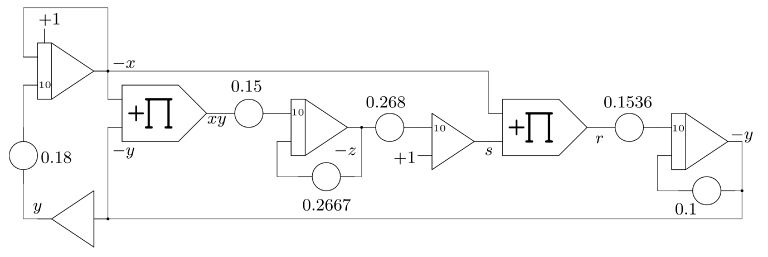
-x=-∫1.8y-x dt+C
-z=-∫1.5xy-0.2667z dt
s=-(1-2.68z)
r=-xs
-y=-∫1.536r-0.1y dt
These equations can now be implemented directly on an analog computer as shown in this program:
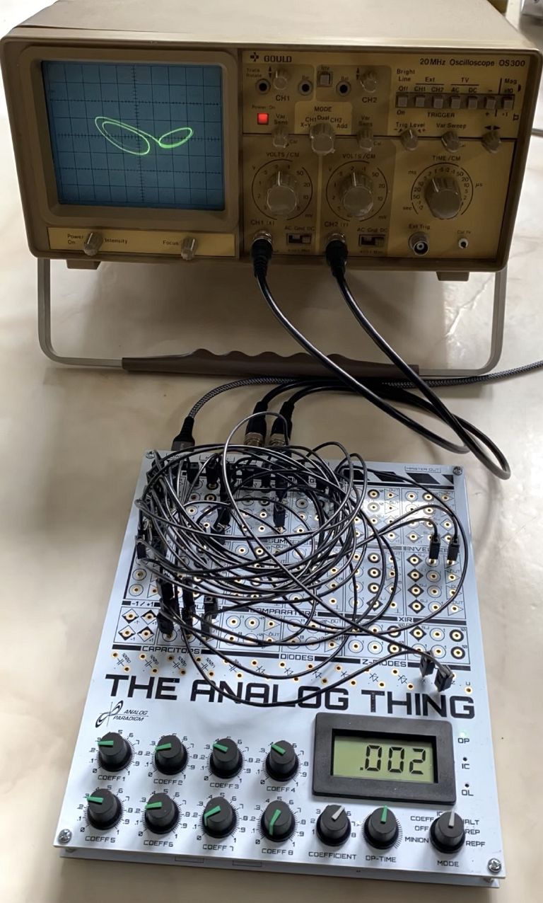
A typical setup looks like this:
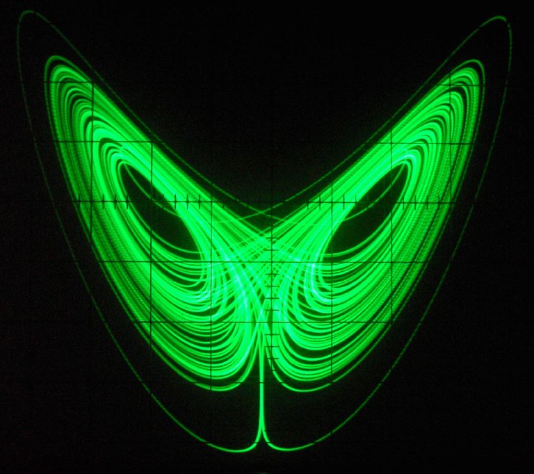
Using a classic analog oscilloscope in xy-mode and a camera capable of long term exposures, the beauty of this particular chaotic attractor can be captured. Shown in the following is the phase space plot of the variables -x and s:
Since THAT offers two time constants for its integrators it is possible to slow down the computation by a factor of 100 by connecting the SLOW jack of every integrator to the output jack of the same integrator. Thus it is possible to control a classic plotter:


