Difference between revisions of "SEIR"
| Line 16: | Line 16: | ||
[[File:SEIR_setup.jpg|512px]] | [[File:SEIR_setup.jpg|512px]] | ||
| + | |||
| + | β, α, γ, and I(0) are represented by the coefficient potentiometers 1, 2, 3, and 4 respectively. | ||
| + | |||
| + | A typical simulation result looks like this screenshot from a four-channel oscilloscope: | ||
| + | |||
| + | [[File:SEIR_result_2_small.jpg|512.px]] | ||
Revision as of 17:26, 17 August 2021
In this example a simple SEIR-model of an infectious disease is setup. This is a classical model with four time varying variables representing the set of susceptible, exposed, infected, and recovered persons.
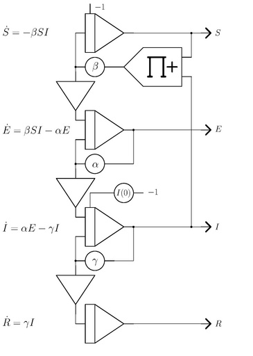
The model is described by four coupled differential equations, one for each of the four variables. Initially, all persons are susceptible in a simulation as they have not been exposed to the disease yet. The number of susceptible persons is computed by the topmost integrator in the program shown below. This integrator has an initial condition of -1 thus yielding S=+1 initially.
The parameter β basically represents the probability of a susceptible person meeting an infected person. (Social distancing would decrease β for example.) The first derivative of S with respect to time (denoted by a dot on top of the variable S) is thus -βSI.
A formerly susceptible person which has been exposed to an infected person is thus removed from the set of susceptible persons and becomes an exposed person E. So the time derivative of E has one term βSI increasing E. Exposed persons become infected persons at a rate determined by α yielding a second term to the time derivative of E.
Accordingly I is increased at the rate αE and decreased at the rate γI which represents recovered (or removed if they might have died) persons. The parameter I(0) represents the number of infected persons at the start of the simulation run.
The number of recovered/removed persons R is increased by γI accordingly.
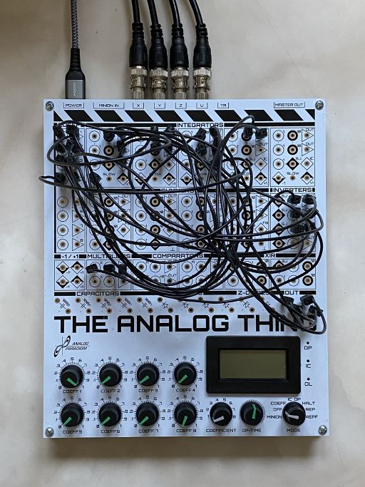
The actual setup of this program on a THAT looks like this:
β, α, γ, and I(0) are represented by the coefficient potentiometers 1, 2, 3, and 4 respectively.
A typical simulation result looks like this screenshot from a four-channel oscilloscope:


