Warning: This simulation requires ten integrators, 15 summers, 16 multipliers, and 17 coefficient potentiometers (-> eight THATs).*
|
|
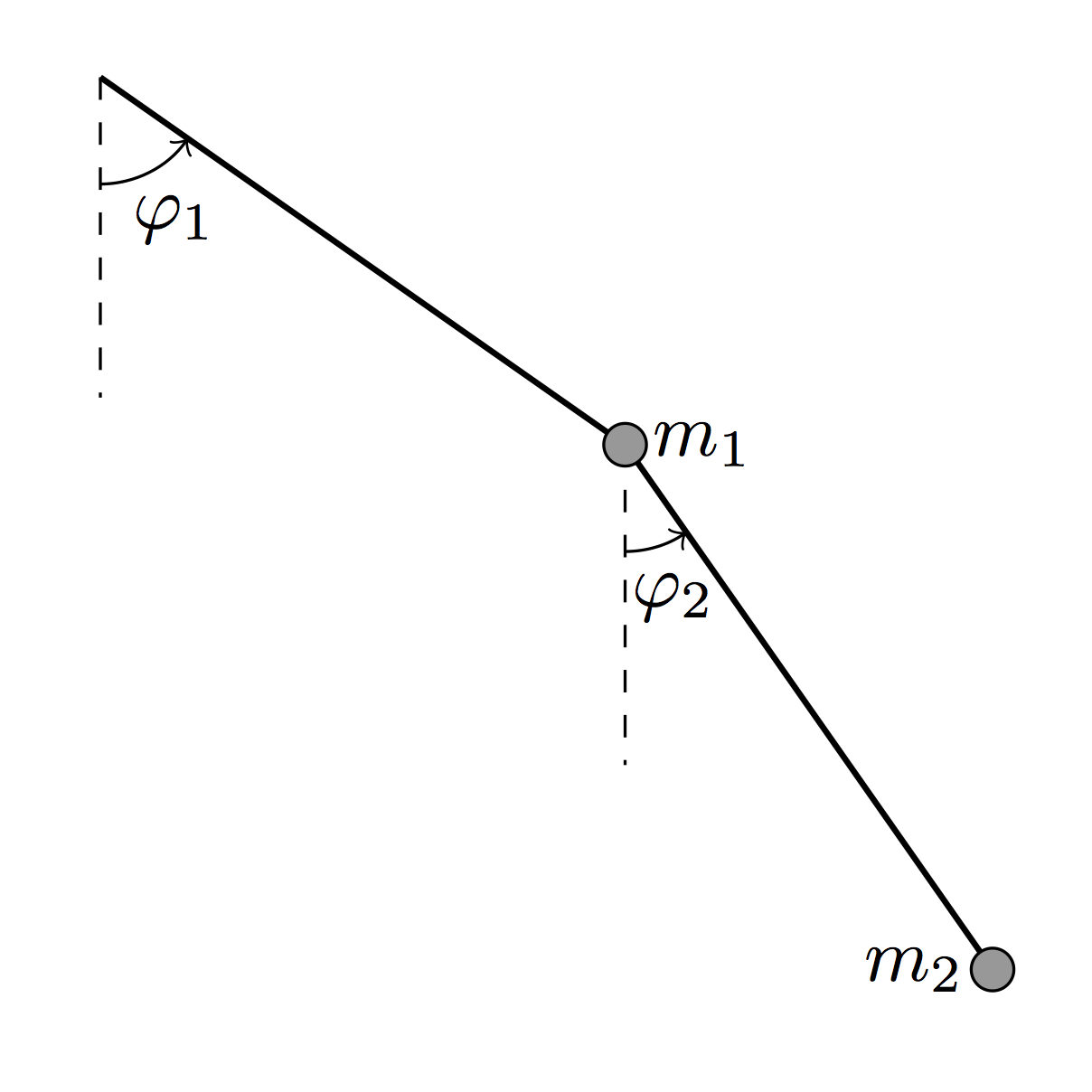
Figure 1: Double pendulum |
This application note describes the simulation of a double pendulum as
shown in figure 1 on an analog computer.
The equations of motion will be derived by determining the Lagrangian
\(L=T-V\) with the two generalized coordinates \(\varphi_1\) and
\(\varphi_2\) where \(T\) represents the total kinetic energy
while \(V\) is the potential energy of the system. This potential
energy is just
(1)\[V=-g\left((m_1+m_2)l_1\cos(\varphi_1)+m_2l_2\cos(\varphi_2)\right)\label{equ_dp_potential_energy}\]
with \(m_1\) and \(m_2\) representing the masses of the two bobs
mounted on the tips of the two pendulum rods (which are assumed as being
weightless). As always, \(g\) represents the gravitational
acceleration.
To derive the total kinetic energy the positions of the pendulum arm
tips \((x_1,y_1)\) and \((x_2,y_2)\) are required:
\[\begin{split}\begin{aligned}
x_1&=l_1\sin(\varphi_1)\\
y_1&=l_1\cos(\varphi_1)\\
x_2&=l_1\sin(\varphi_1)+l_2\sin(\varphi_2)\\
y_2&=l_1\cos(\varphi_1)+l_2\cos(\varphi_2)
\end{aligned}\end{split}\]
The first derivatives of these with respect to time are
\[\begin{split}\begin{aligned}
\dot{x}_1&=\dot{\varphi}_1l_1\cos(\varphi_1),\\
\dot{y}_1&=-\dot{\varphi}_1l_1\sin(\varphi_1),\\
\dot{x}_2&=\dot{\varphi}_1l_1\cos(\varphi_1)+\dot{\varphi}_2l_2\cos(\varphi_2)\text{~and}\\
\dot{y}_2&=-\dot{\varphi}_1l_1\sin(\varphi_1)-\dot{\varphi}_2l_2\sin{\varphi_2}.
\end{aligned}\end{split}\]
The kinetic energy of the system is then
(2)\[T=\frac{1}{2}\left(m_1(\dot{x}_1^2+\dot{y}_1^2)+m_s(\dot{x}_2^2+\dot{y}_2^2)\right)\label{equ_dp_kinetic_energy}\]
with
\[\begin{split}\begin{aligned}
\dot{x}_1^2&=\dot{\varphi}_1^2l_1^2\cos^2(\varphi_1)\\
\dot{y}_1^2&=\dot{\varphi}_1^2l_1^2\sin^2(\varphi_1)\\
\dot{x}_2^2&=\dot{\varphi}_1^2l_1^2\cos^2(\varphi_1)+2\dot{\varphi}_1\dot{\varphi}_2l_1l_2\cos(\varphi_1)\cos(\varphi_2)+\dot{\varphi}_2^2l_2^2\cos^2(\varphi_2)\\
\dot{y}_2^2&=\dot{\varphi}_1^2l_1^2\sin^2(\varphi_1)+2\dot{\varphi}_1\dot{\varphi}_2l_1l_2\sin(\varphi_1)\sin(\varphi_2)+\dot{\varphi}_2^2l_2^2\sin^2(\varphi_2)
\end{aligned}\end{split}\]
and thus
(3)\[\begin{split}\begin{aligned}
\dot{x}_1^2+\dot{y}_1^2&=\dot{\varphi}_1^2l_1^2\cos^2(\varphi_1)+\varphi_1^2l_1^2\sin^2(\varphi_1)\nonumber\\
&=\dot{\varphi}_1^2l_1^2\left(\cos^2(\varphi_1)+\sin^2(\varphi_1)\right)\nonumber\\
&=\dot{\varphi}_1^2l_1^2\label{equ_dp_sp_1}\\
\end{aligned}\end{split}\]
(4)\[\begin{split}\begin{aligned}
\dot{x}_2^2+\dot{y}_2^2&=\dot{\varphi}_1^2l_1^2\left(\cos^2(\varphi_1)+\sin^2(\varphi_1)\right)+\dot{\varphi}_2^2l_2^2\left(\cos^2(\varphi_2)+\sin^2(\varphi_2)\right)+\nonumber\\
&~~~~2\dot{\varphi}_1\dot{\varphi}_2l_1l_2\left(\cos(\varphi_1)\cos(\varphi_2)+\sin(\varphi_1)\sin(\varphi_2)\right)\nonumber\\
&=\dot{\varphi}_1^2l_1^2+\dot{\varphi}_2^2l_2^2+2\dot{\varphi}_1\dot{\varphi}_2l_1l_2\cos(\varphi_1-\varphi_2)\label{equ_dp_sp_2}
\end{aligned}\end{split}\]
The Lagrangian \(L\) results from equations (1) and (2) with (3) and (4) as
(5)\[\begin{split}\begin{aligned}
L&=\frac{1}{2}l_1^2\dot{\varphi}_1^2(m_1+m_2)+\frac{1}{2}m_2\dot{\varphi}_2^2l_2^2+m_2\dot{\varphi}_1\dot{\varphi}_2l_1l_2\cos(\varphi_1-\varphi_2)+\nonumber\nonumber\\
&~~~~g(m_1+m_2)l_1\cos(\varphi_1)+gm_2l_2\cos(\varphi_2).\label{equ_dp_lagrangian}
\end{aligned}\end{split}\]
Now the Euler-Lagrange-equations
(6)\[\begin{split}\begin{aligned}
\frac{\text{d}}{\text{d}t}\frac{\partial L}{\partial\dot{\varphi}_1}-\frac{\partial L}{\partial\varphi_1}&=0\label{equ_dp_eula_1}\\
\end{aligned}\end{split}\]
and
(7)\[\begin{aligned}
\frac{\text{d}}{\text{d}t}\frac{\partial L}{\partial\dot{\varphi}_2}-\frac{\partial L}{\partial\varphi_2}&=0\label{equ_dp_eula_2}
\end{aligned}\]
have to be solved. The required (partial) derivatives are
\[\begin{split}\begin{aligned}
\frac{\partial L}{\partial\varphi_1}&=-m_2\dot{\varphi}_1\dot{\varphi}_2l_1l_2\sin(\varphi_1-\varphi_2)-g(m_1+m_2)l_1\sin(\varphi_1)\\
\frac{\partial L}{\partial\dot{\varphi}_1}&=l_1^2\dot{\varphi}_1(m_1+m_2)+m_2\dot{\varphi}_2l_1l_2\cos(\varphi_1-\varphi_2)\\
\frac{\text{d}}{\text{d}t}\frac{\partial L}{\partial\dot{\varphi}_1}&=l_1^2\ddot{\varphi}_1(m_1+m_2)+m_2l_1l_2\left[\ddot{\varphi}_2\cos(\varphi_1-\varphi_2)-\dot{\varphi}_2\sin(\varphi_1-\varphi_2)(\dot{\varphi}_1-\dot{\varphi}_2)\right]\\
\frac{\partial L}{\partial\varphi_2}&=m_2\dot{\varphi}_1\dot{\varphi}_2l_1l_2\sin(\varphi_1-\varphi_2)-gm_2l_2\sin(\varphi_2)\\
\frac{\partial L}{\partial\dot{\varphi}_2}&=m_2\dot{\varphi}_2l_2^2+m_2\dot{\varphi}_1l_1l_2\cos(\varphi_1-\varphi_2)\\
\frac{\text{d}}{\text{d}t}\frac{\partial L}{\partial\dot{\varphi}_2}&=m_2\ddot{\varphi}_2l_2^2+m_2l_1l_2\left[\ddot{\varphi}_1\cos(\varphi_1-\varphi_2)-\dot{\varphi}_1\sin(\varphi_1-\varphi_2)(\dot{\varphi}_1-\dot{\varphi}_2)\right].
\end{aligned}\end{split}\]
based on (5). Substituting
these into (6) yields
\[\begin{split}\begin{aligned}
0&=l_1^2\ddot{\varphi}_1(m_1+m_2)-m_2l_1l_2\ddot{\varphi}_2\cos(\varphi_1-\varphi_2)-m_2l_1l_2\dot{\varphi}_2\sin(\varphi_1-\varphi_2)(\dot{\varphi}_1-\dot{\varphi}_2)+\\
&~~~~m_2\dot{\varphi}_1\dot{\varphi}_2l_1l_2\sin(\varphi_1-\varphi_2)+gl_1(m_1+m_2)\sin(\varphi_1).
\end{aligned}\end{split}\]
Expanding \((\dot{\varphi}_1-\dot{\varphi}_2)\) yields
\[\begin{split}\begin{aligned}
0&=l_1^2\ddot{\varphi}_1(m_1+m_2)+m_2l_1l_2\ddot{\varphi}_2\cos(\varphi_1-\varphi_2)+\\
&~~~~m_2l_1l_2\dot{\varphi}_2^2\sin(\varphi_1-\varphi_2)+gl_1(m_1+m_2)\sin(\varphi_1).
\end{aligned}\end{split}\]
Dividing by \(l_1^2(m_1+m_2)\) results in
\[0=\ddot{\varphi}_1+\frac{m_2}{m_1+m_2}\frac{l_2}{l_1}\ddot{\varphi}_2\cos(\varphi_1-\varphi_2)+\frac{m_2}{m_1+m_2}\frac{l_2}{l_1}\dot{\varphi}_2^2\sin(\varphi_1-\varphi_2)+\frac{g}{l_1}\sin(\varphi_1)\]
which can be further simplified as
(8)\[0=\ddot{\varphi}_1+\frac{m_2}{m_1+m_2}\frac{l_2}{l_1}\left[\ddot{\varphi}_2\cos(\varphi_1-\varphi_2)+\dot{\varphi}_2^2\sin(\varphi_1-\varphi_2)\right]+\frac{g}{l_1}\sin(\varphi_1).\label{equ_dp_motion_1}\]
Proceeding analogously, (7) yields
(9)\[0=\ddot{\varphi}_2+\frac{l_1}{l_2}\left[\ddot{\varphi}_1\cos(\varphi_1-\varphi_2)-\dot{\varphi}_1^2\sin(\varphi_1-\varphi_2)\right]+\frac{g}{l_2}\sin(\varphi_2)\label{equ_dp_motion_2}\]
after some rearrangements.
To simplify things further it will be assumed that \(m_1=m_2=1\) and \(l_1=l_2=1\)
in arbitrary units yielding the following two equations of motion of the double pendulum based on
(8) and
(9):
\[\begin{split}\begin{aligned}
\ddot{\varphi}_1&=-\frac{1}{2}\left[\ddot{\varphi}_2\cos(\varphi_1-\varphi_2)+\dot{\varphi}_2^2\sin(\varphi_1-\varphi_2)+2g\sin(\varphi_1)\right]\label{equ_dp_motion_1_final}\\
\ddot{\varphi}_2&=-\left[\ddot{\varphi_1}\cos(\varphi_1-\varphi_2)-\dot{\varphi}_1^2\sin(\varphi_1-\varphi_2)+g\sin(\varphi_2)\right]\label{equ_dp_motion_2_final}
\end{aligned}\end{split}\]
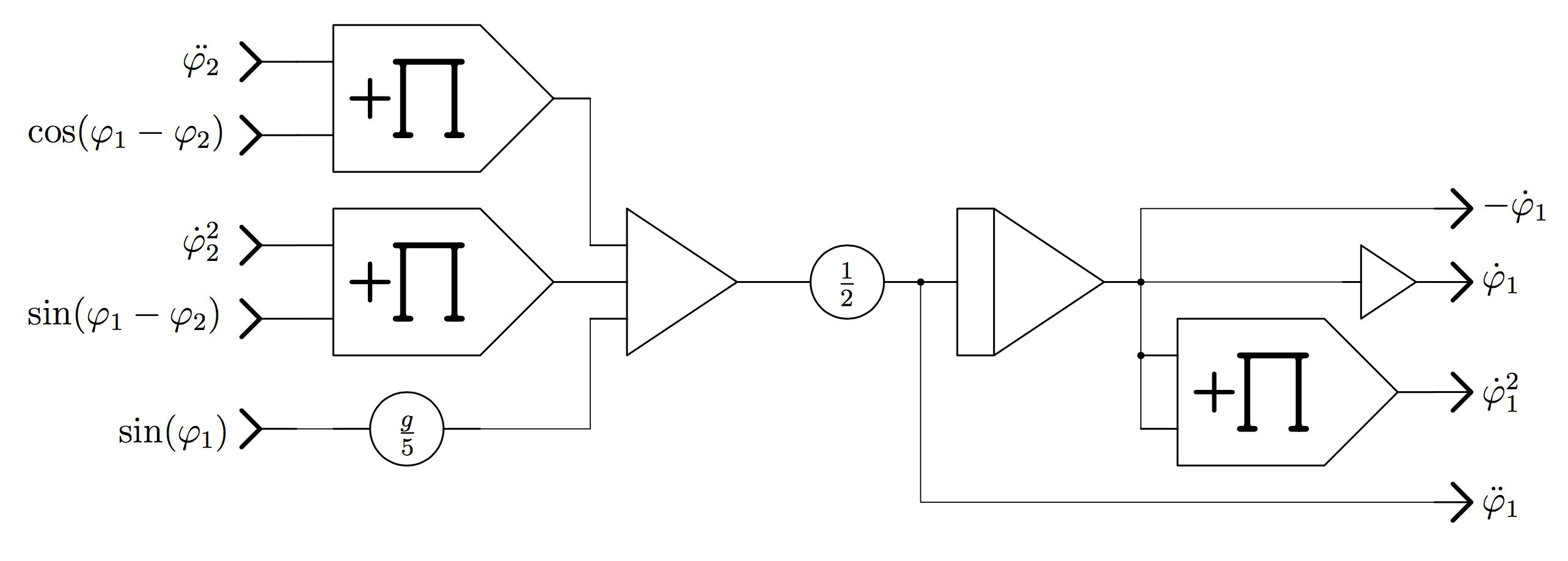
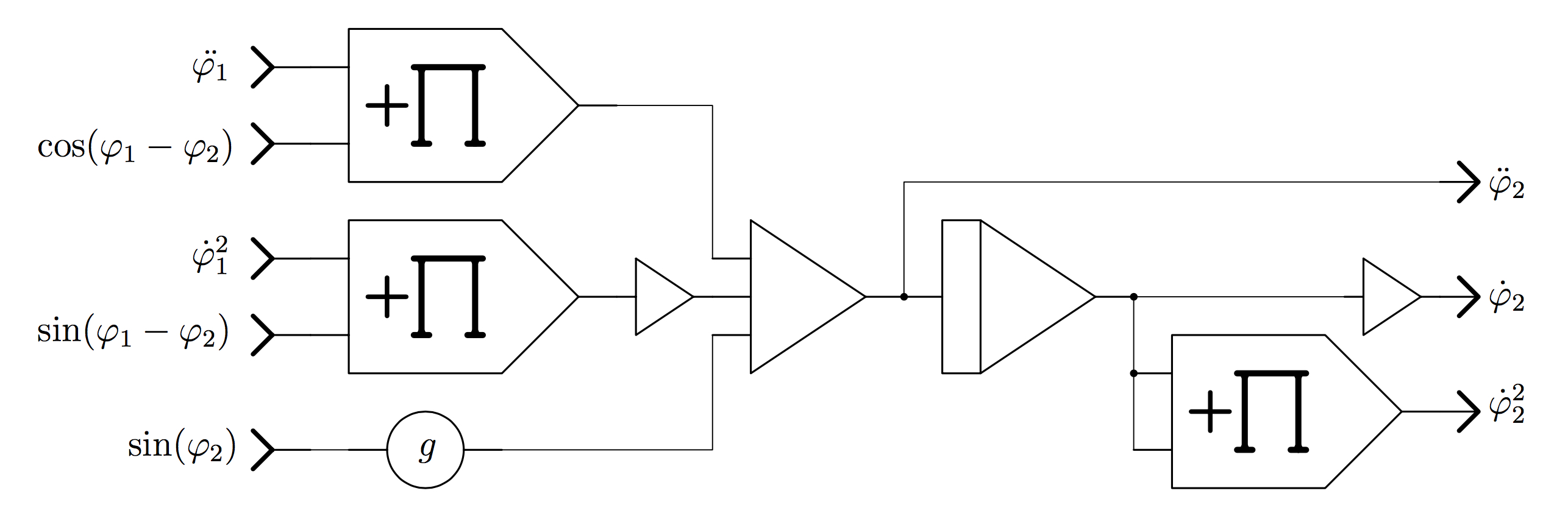
The implementation of equations
(10) and (11) is straightforward as shown in figures 2 and 3. Both circuits require
the functions \(\sin(\varphi_1-\varphi_2)\),
\(\cos(\varphi_1-\varphi_2)\), \(\sin(\varphi_1)\), and
\(\sin(\varphi_2)\), which are generated by three distinct
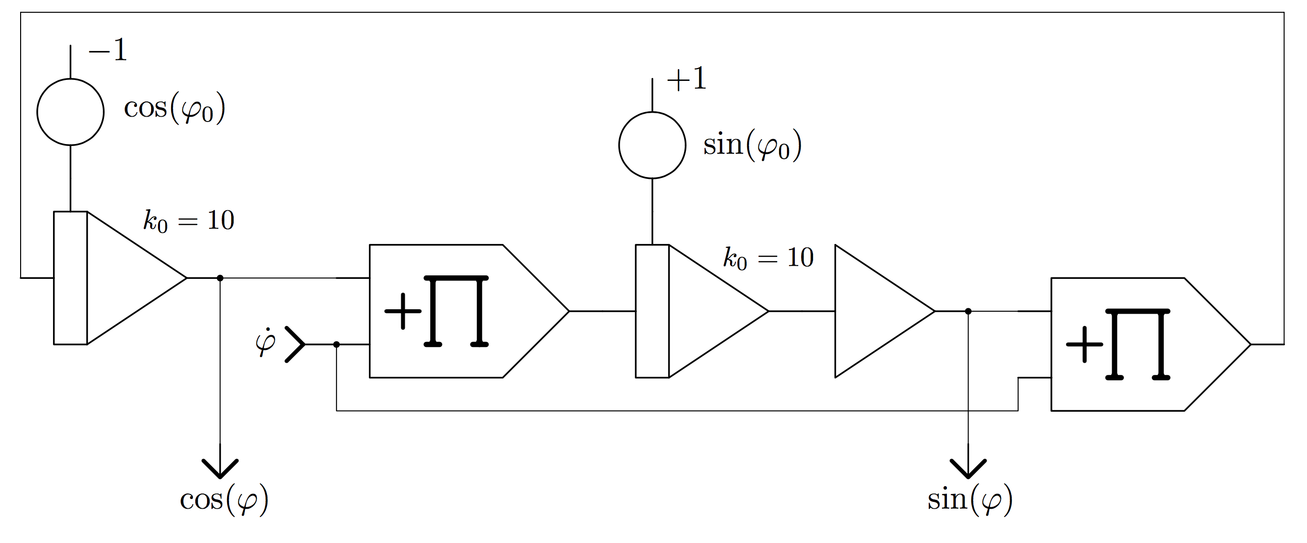
sub-circuits such as the one shown in figure 4. These circuits yield
sine and cosine of an angle based on the first time-derivative of this
angle, so the simulation is not limited to a finite range for the two
angles \(\varphi_1\) and \(\varphi_2\).
It should be noted that each of the two integrators of each of these
three harmonic function generators has a potentiometer connected to its
respective initial value input. When a simulation run with given initial
values for \(\varphi_1(0)\) and \(\varphi_2(0)\) is to be
started, these potentiometers have to be set to
\(\cos(\varphi_1(0))\), \(\sin(\varphi_1(0))\) and
\(\cos(\varphi_2(0))\), \(\sin(\varphi_2(0))\), respectively.
|
|
|
Figure 2: Implementation of equation (10) |
Figure 3: Implementation of equation (11) |
Since \(\dot{\varphi}_1\) and \(\dot{\varphi}_2\) are readily
available from the circuits shown in figures 2 and 3, two of these harmonic
function generators can be directly fed with these values. The input for
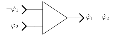
the third function generator is generated by a two-input summer as shown in figure 5.
|
|
|
Figure 4: Generating sin(\(\varphi\)) and cos(\(\varphi\)) |
Figure 5: Computing \({\dot{\varphi}_1}\) - \({\dot{\varphi}_2}\) |
|
|
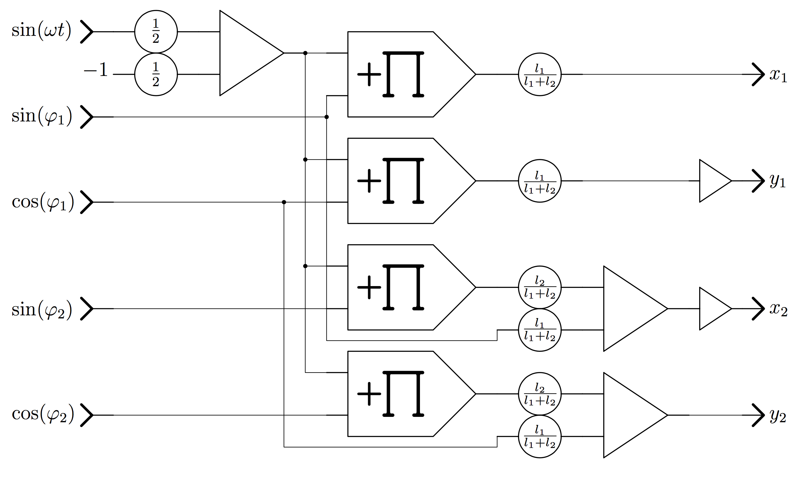
Figure 6: Display circuit for the double pendulum |
With \(\dot{\varphi}_1\) and \(\dot{\varphi}_2\) and thus
\(\sin(\varphi_1)\), \(\cos(\varphi_1)\), and
\(\sin(\varphi_2)\), \(\cos(\varphi_2)\) readily available, the
double pendulum can be displayed on an oscilloscope featuring two
separate \(x,y\)-inputs by means of the circuit shown in figure 6. To yield a flicker-free display,
this circuit requires a high-frequency input \(\sin(\omega t)\)
which can be obtained by two integrators in series with a summer, the
output of which is fed back into the first integrators. This circuit is
not shown here but can be found in [ULMANN 2017, p.67].
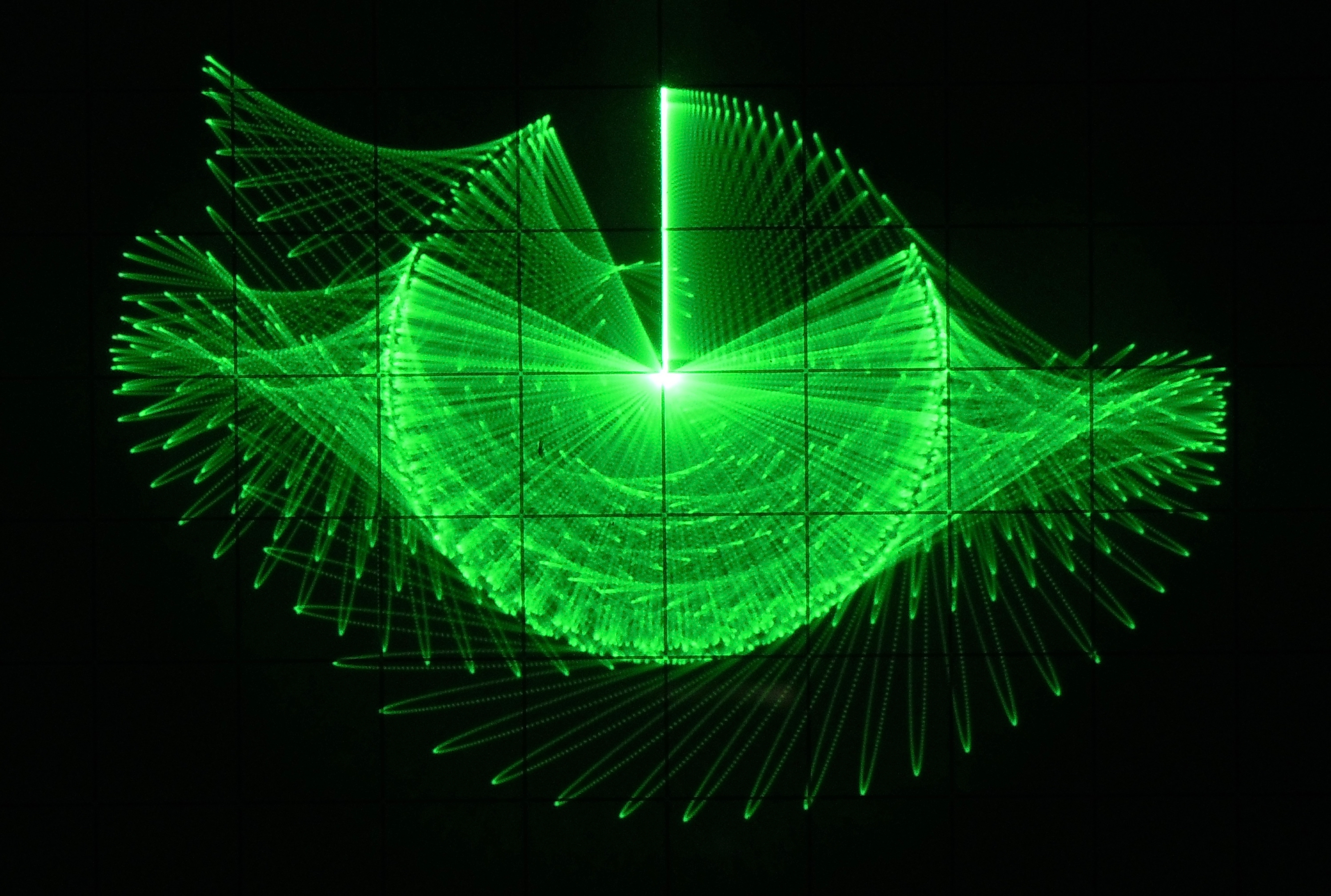
Figure 7 shows a long-term exposure
of the movements of the double pendulum starting as an inverted pendulum
with its first pendulum rod pointing upwards while the second one points
downwards.
|
|
Figure 7: Long-term exposure of a double pendulum simulation run |
This simulation requires ten integrators, 15 summers, 16 multipliers,
and 17 coefficient potentiometers.
[MAHRENHOLTZ, 1968] Oskar Mahrenholtz, Analogrechnen in Maschinenbau und Mechanik, BI
Hochschultaschenbücher, 1968
[Ulmann 2017] Bernd Ulmann, Analog Computer
Programming, Create Space, 2017