Quantum Mechanical Two-Body Problem with Gaussian potential
Contents
Quantum Mechanical Two-Body Problem with Gaussian potential
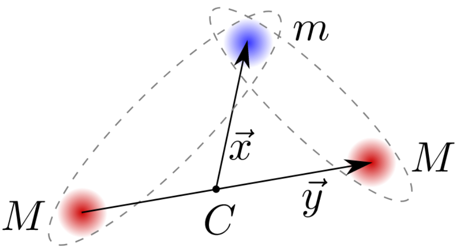
Figure 1: Two heavy (M) particles and one light (m) particle in a three-body system
This application note is inspired by the work described in [Thies et al. 2022]. In this paper the authors develop a numerical method to calculate binding energies of a quantum mechanical three-body system efficiently. This three-body system is composed of two heavy and one light particle. In figure 1 the system is displayed with its two-body (heavy/light) subsystems marked by dashed ellipses. The routine to calculate binding energies for the three-body system first solves the two-body subsystem. This application note aims to reproduce the findings in for the two-body systems using an analog computer.
Implementation
The Schrödinger equation for the two-body system is given by
where \(\xi\) is the distance between the two particles, \(E\) their energy, \(\psi(\xi)\) the wave function of the system, \(-v_0f(\xi)\) an attractive potential between the particles, and \(\Delta_\xi\) the Laplace operator. The depth of the potential is given by \(v_0\) and the shape is defined by a Gaussian function
With a Gaussian potential equation (1) becomes symmetric under the transformation \(\xi \rightarrow -\xi\) and the solutions are either even (\(\psi(\xi) = \psi(-\xi)\)) or odd (\(\psi(-\xi) = -\psi(\xi)\)). Hence, equation (1) can be solved for \(\xi>0\) with initial conditions of either \(\psi(0)\neq 0\) and \(\psi'(0) = 0\) (even) or \(\psi(0) = 0\) and \(\psi'(0)\neq 0\) (odd).
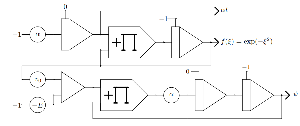
Figure 2: Analog computer program solving the Schr ̈odinger equation with Gaussian potential.
In figure 2 the analog program to solve equation (1) is shown. In the upper half the Gaussian function is generated by solving the differential equation
One has to be careful about the variable of interest in equations such as (3) because \(\frac{\text{d}}{\text{d}\xi} \neq \frac{\text{d}}{\text{d}t}\) (all integrators integrate over time).
In the following \(\xi\) is defined as \(\xi = \sqrt{\frac{\alpha}{2}} t\), implying \(\frac{\text{d}}{\text{d}\xi} = \sqrt{\frac{2}{\alpha}} \frac{\text{d}}{\text{d}t}\). With this eq. (3) can be rewritten as
The implementation of eq. (4) can directly be seen in the upper half of the analog program in figure 2. The lower half implements the two-body Schrödinger equation in eq. (1). To see this correspondence the equation can be rewritten:
The implementation of eq. (7) in the lower half of figure (2) is straightforward. The potentiometer for \(E\) gets a negative reference input since for a positive potential depth \(v_0>0\) the wave function \(\psi\) is only bound if the energy is negative. The initial conditions for \(\psi\) in figure (2) are set to generate even solutions.
Calculation
In binding energies for the three-body system are calculated for values of the potential depth \(v_0\) for which the two-body subsystem has specific energy values. So for a given energy one is interested in the value of \(v_0\), or in other words the strength of the attractive force between the two particles, for which the two-body system is bound.
A system is in a bound state, if its wave function \(\psi\) remains localized. This implies that for large values of \(\xi\), \(\psi\) tends to zero (\(\lim_{\xi\rightarrow \pm \infty} \psi(\xi) = 0\)). In the following two-body energies of \(E=-10^{-1},-10^{-2},-10^{-3}\) are investigated. The potential depth \(v_0\) required for the system to be in a bound state can be derived by varying \(v_0\) until \(\psi\) is localized.
This process in depicted in figure 3. The program is set up for \(E=-0.1\) and \(\alpha=0.1\) on an Analog Paradigm Model-1. All integrators have a time scale factor of \(k_0 = 10^4\) with the exception of two integrators with an \(\alpha=0.1\) scaling in front, which is absorbed into the time scale factor by setting \(k_0 = 10^3\). With this setup the effect on \(\psi\) by varying \(v_0\) can be tested and a bound state of the system can be derived.
|
|
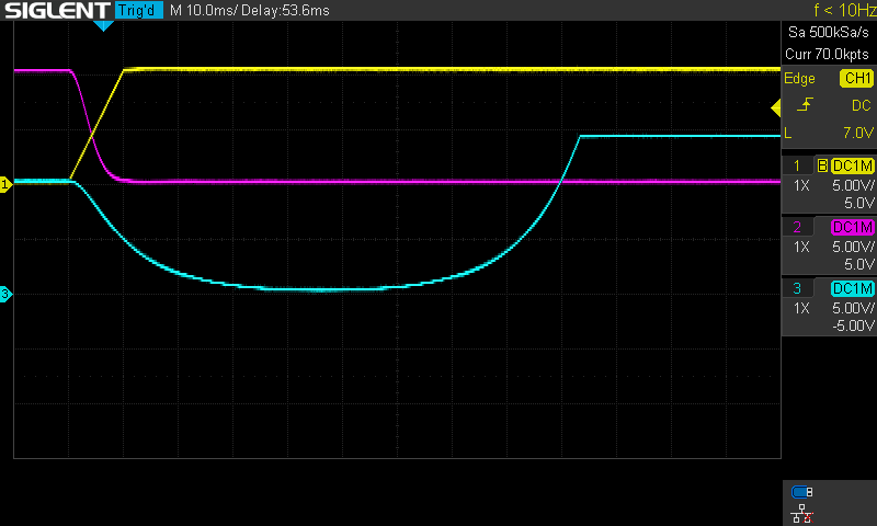
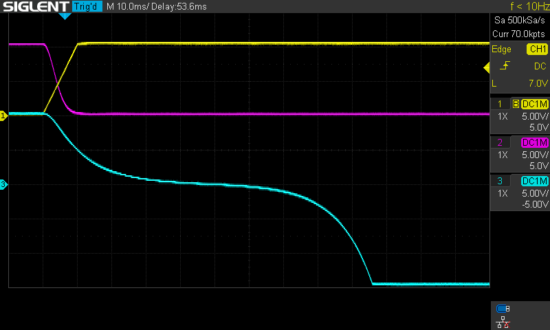
Figure 3: Two runs of the analog program for E = −0.1 and α = 0.1
In figure 3 it can be seen that even very slight changes of \(v_0\) affect \(\psi\). Both of the states are not bound states, because \(\lim_{\xi\rightarrow \pm \infty} \psi(\xi) \neq 0\). However, the two states in figure 3 suggest that for some value of \(v_0\) between \(0.342\) and \(0.343\) there is a bound state. With this process regions of \(v_0\) for different values of \(E\), in which the system is bound, can be derived.
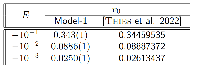
Table 1: Values of v0 at different energies E. Results from the Model-1 analog computer are compared with results from [Thies et al. 2022].
Results
In table 1 the results from the analog computer are compared with the results in . The values of \(v_0\) derived by the analog computer setup are all close the theoretical values. For \(E=-0.1\) and \(E=-0.01\) the deviations are less than \(0.5\%\) and for \(E=-10^{-3}\) it is about \(5\%\). The uncertainties given for values of \(v_0\) from the Model-1 are derived from the variation of \(v_0\) around the bounded state of \(\psi\). Uncertainties of the analog program due to the limited precision of analog components are not analysed.
References
[Thies et al. 2022] Jonas This, Moritz Travis Hof, Matthias Zimmermann, Maxim Efremov, “Tensor Product Scheme for Computing of Bound States of the Quantum Mechanical Three-Body Problem”, https://arxiv.org/pdf/2111.02534.pdf, 2022