Contents
Sprott SQM model
This application note implements the \(SQ_M\) model (cf. ), an example of a simple three-dimensional chaotic flow with a quadratic nonlinearity. The model consists of three coupled differential equations
with \(\alpha=1.7\) and the initial conditions \(x(0)=1, y(0)=-0.8, z(0)=0\). To scale the system, three scale factors \(\lambda_x=\lambda_z=\frac{1}{4}\) and \(\lambda_y=\frac{1}{6}\) are introduced which in turn yield (after collecting all resulting factors)
Thanks to the constant term \(\frac{\alpha}{4}\), the initial conditions mentioned in the original system can be safely ignored as it will enter its chaotic oscillation right away.
The analog computer setup can be derived directly from the scaled equations (1), (2) and (3) as shown in figure 1.
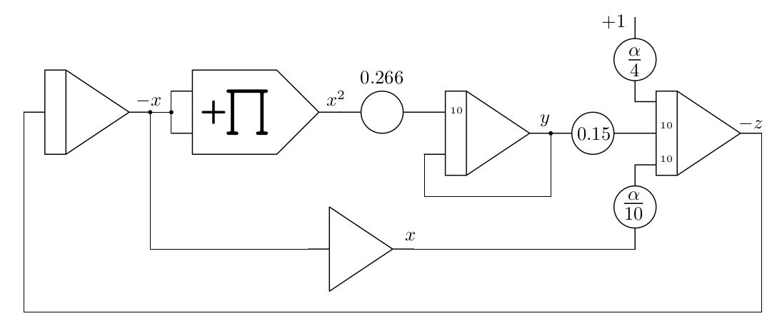
|
Figure 1: Analog computer setup for the SQM model |
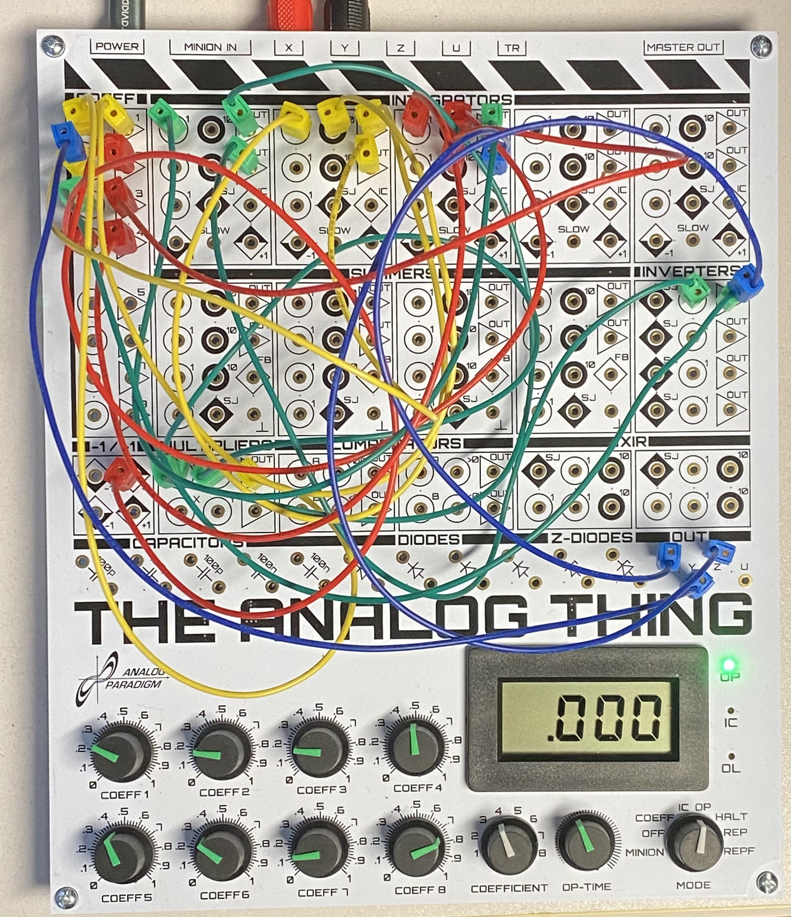
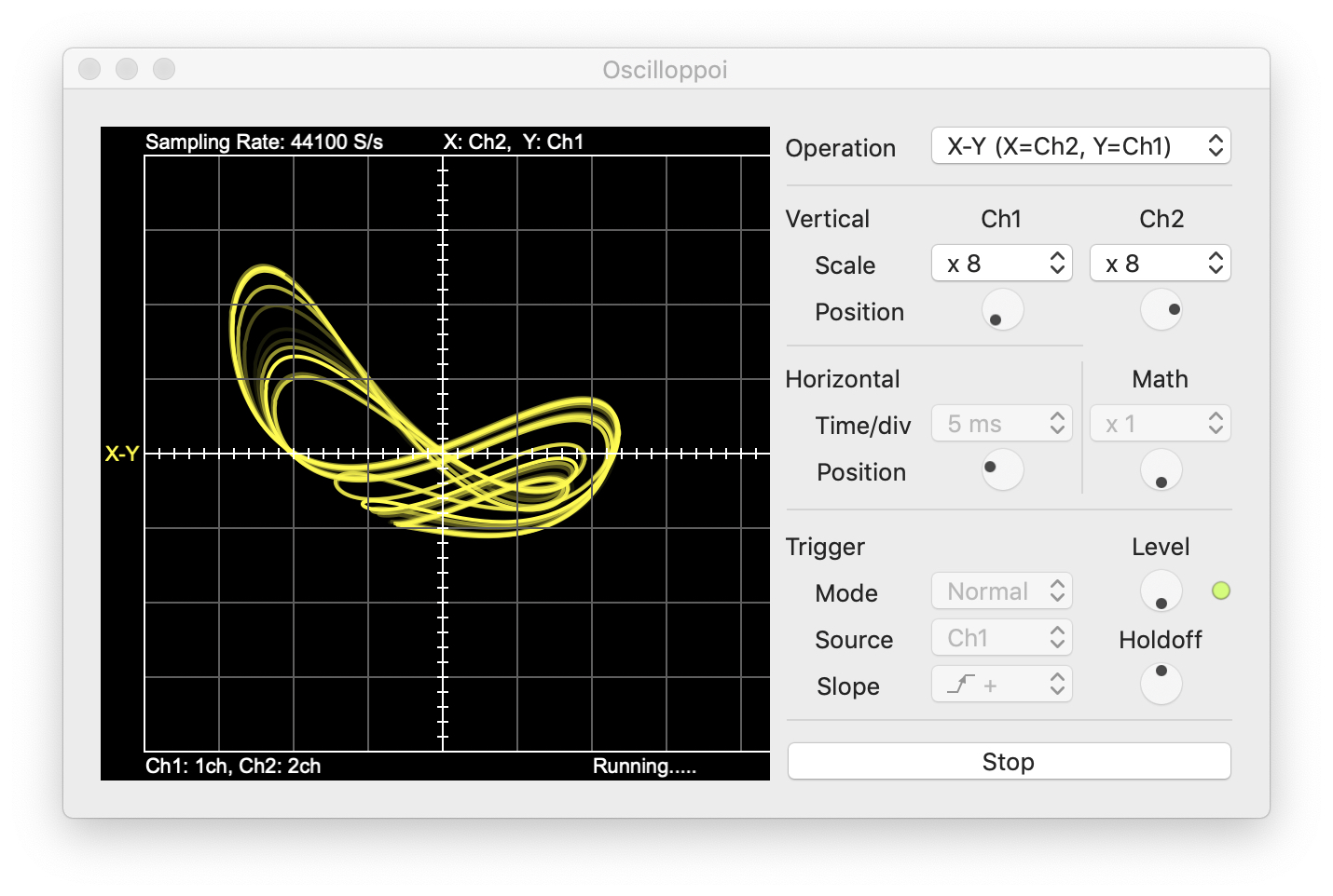
This little program is ideally suited for THE ANALOG THING as can be seen in figure 2. Figure 3 shows a typical phase space plot of \(x\) vs. \(y\) which was caputured using a USB-soundcard with stereo line in and the software Oscilloppoi 1 running on a Mac.
|
|
Figure 2: Implementation of the program shown in figure 1 |
Figure 3: xy phase space plot of the SQ M system |
References
[Sprott(2016)] Julien Clinton Sprott, Elegant Chaos – Algebraically Simple Chaotic Flows, World Scientific, 2016