Contents
Lorenz-attractor 1
Introduction
This issue 2 of “Analog Computer Applications” deals with one of the most intriguing and well known chaotic attractors, the so-called Lorenz-attractor or -system. It was developed in 1963 by Edward Norton Lorenz 2 as a simplified model for atmospheric convection and first described in . Although this seminal work was performed on a digital computer, a Royal McBee LGP-30, the Lorenz-attractor is ideally suited to be implemented on an analog computer.
Scaling
This dynamic chaotic attractor is described by three coupled differential equations of the form 3
where \(\sigma=10, \beta=\frac{8}{3}\), and \(\rho=28\). Obviously, this set of DEQs is not directly suitable for an analog computer as it is not properly scaled. Scaling the equations of systems like this is not a trivial task. First, the domains of the variables have to be determined. This can either be done manually on an analog computer, starting with unscaled equations and running until an overload condition arises. Then the offending variable is determined and a guesstimated scale factor for this particular variable introduced. Alternatively, a digital computer even employing simple integration schemes like the first-order Euler-integration can be used in this step. As soon as minimum/maximum values for the variables are (roughly) determined, the equations can be scaled by introducing appropriate scaling factors.
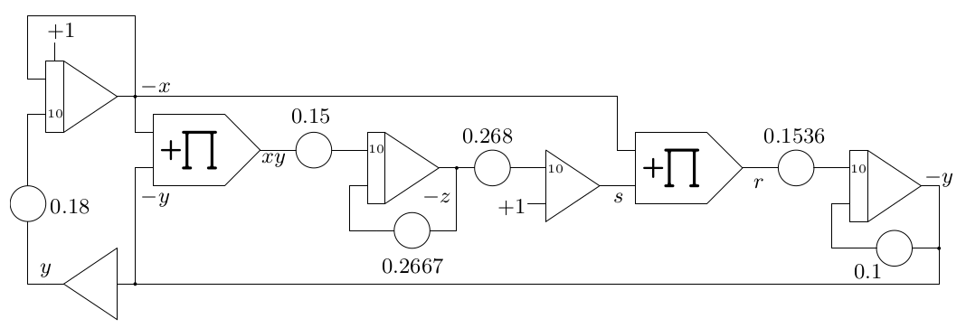
The equations above were transformed and scaled as follows for implementation on an analog computer:
\(C\) denotes the initial condition of the integrator yielding \(x\) and is quite uncritical. Taking into account that every summer and integrator of an analog computer performs an implicit change of sign, and further noting that \(xy=-x(-y)\), these equations can be further simplified a bit, saving two inverters in the resulting computer setup:
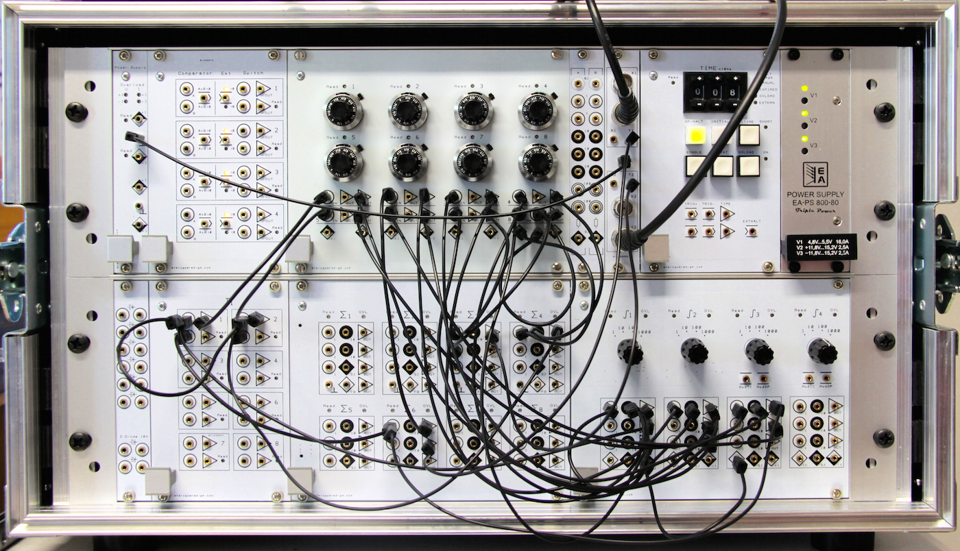
Setup
These equations can now readily implemented on a decent analog computer like the minimal Analog Paradigm Model-1 shown below:
The corresponding schematic looks like this:
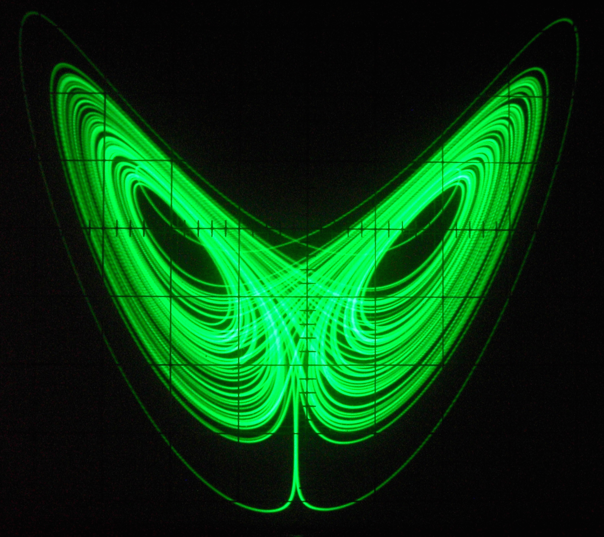
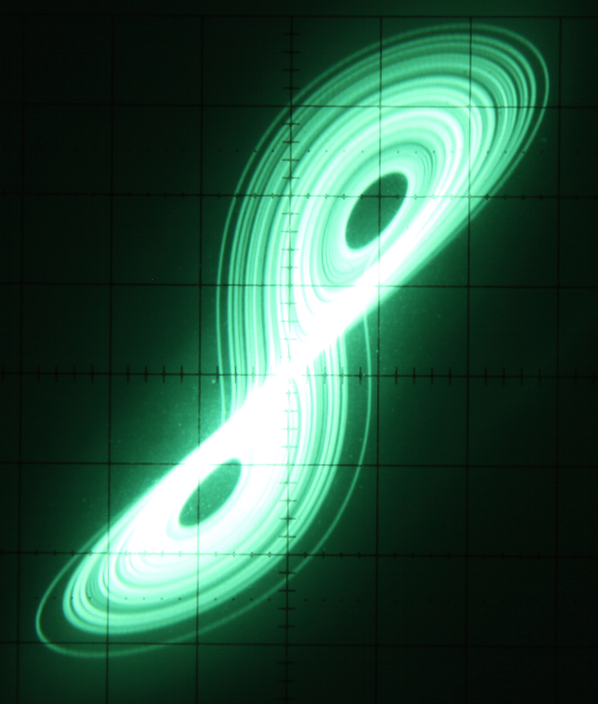
Results
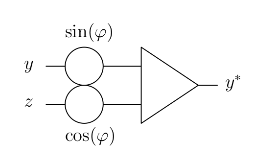
Depending on the time constant \(k_0\) set for the integrators, either a mechanical \(x/y\)-plotter or an oscilloscope may be used to get a graphical representation of this chaotic attractor. The following pictures give some impressions of various projections of this attractor using the following circuit with appropriate values set for \(\sin(\varphi)\) and \(\cos(\varphi)\):
9 Christian Kuehn, Multiple Time Scale Dynamics, Springer, 2015 Edward Norton Lorenz, “Deterministic Nonperiodic Flow”, in Journal of the Atmospheric Sciences, Volume 20, pp. 130–141, March 1963