Contents
The Euler spiral
The first example in the beautiful book is the Euler spiral, which is a clothoid, i. e. a curve with a curvature depending linearly on the arc length. Clothoids play a significant role in road and railway track construction. Imagine driving along a straight road, approaching a curve. If the straight part of the road was directly connected to an arc of a circle forming the curve, one would have to switch from a steering angle of zero to a non-zero steering angle instantaneously, which is impracticable even at rather low speeds. Therefore, a safe curve in a road has a curvature that starts at zero, rises to a maximum and then falls back to zero again when the next straight segment of the road is entered. This can be done by using clothoids and many curves encountered on highways and railway tracks are based on this type of curve.
Generally, a curve parameterized by some functions \(x(t)\), \(y(t)\) has a slope
an arc length
and a curvature
Using the general parameterization
yields the following time derivatives:
Inserting these into (1), (2) and (3) yields
The Euler spiral satisfies \(\kappa=t\), i. e. \(\dot{f}=t\) yielding \(f(t)=\frac{t^2}{2}\) from which its parameterization
follows. This looks pretty straightforward to implement on an analog computer but classic function generators for \(\sin(\varphi)\) and \(\cos(\varphi)\) have a limited interval for \(\varphi\), typically \([-\frac{\pi}{2},\frac{\pi}{2}]\). If more than a very short segment of the Euler spiral is to be generated by an analog computer, a trick must be employed. The idea is to use a quadrature generator 1 which gets \(\dot{\varphi}\) instead of \(\varphi\) as its input. Such a generator, basically consisting of two integrators, two multipliers (to introduce \(\dot{\varphi}\) into the underlying DEQ) and an inverter.
Figure 1 shows the analog computer program for generating an Euler spiral. The quadrature output output signals \(\cos\left(\frac{t^2}{2}\right)\) and \(\sin\left(\frac{t^2}{2}\right)\) are fed to integrators yielding \(x(t)\) and \(y(t)\), while \(\dot{\varphi}\) is obtained by another integrator generating a linear ramp from \(-1\) to \(+1\).
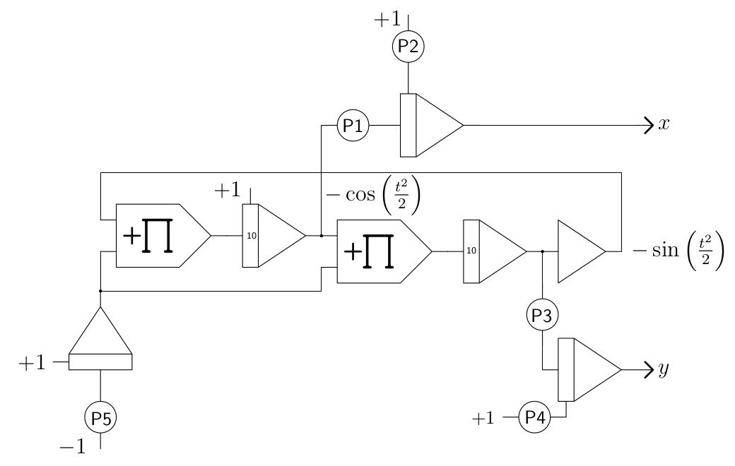
|
Figure 1: Analog computer program for generating an Euler spiral |
Coefficient |
Description |
Typical value |
|---|---|---|
P1 |
\(x\) scaling |
\(0.6\) |
P2 |
\(x\) shift |
\(0.87\) |
P3 |
\(y\) scaling |
\(0.6\) |
P4 |
\(y\) shift |
\(0.75\) |
P5 |
ramp slope |
\(0.1\) |
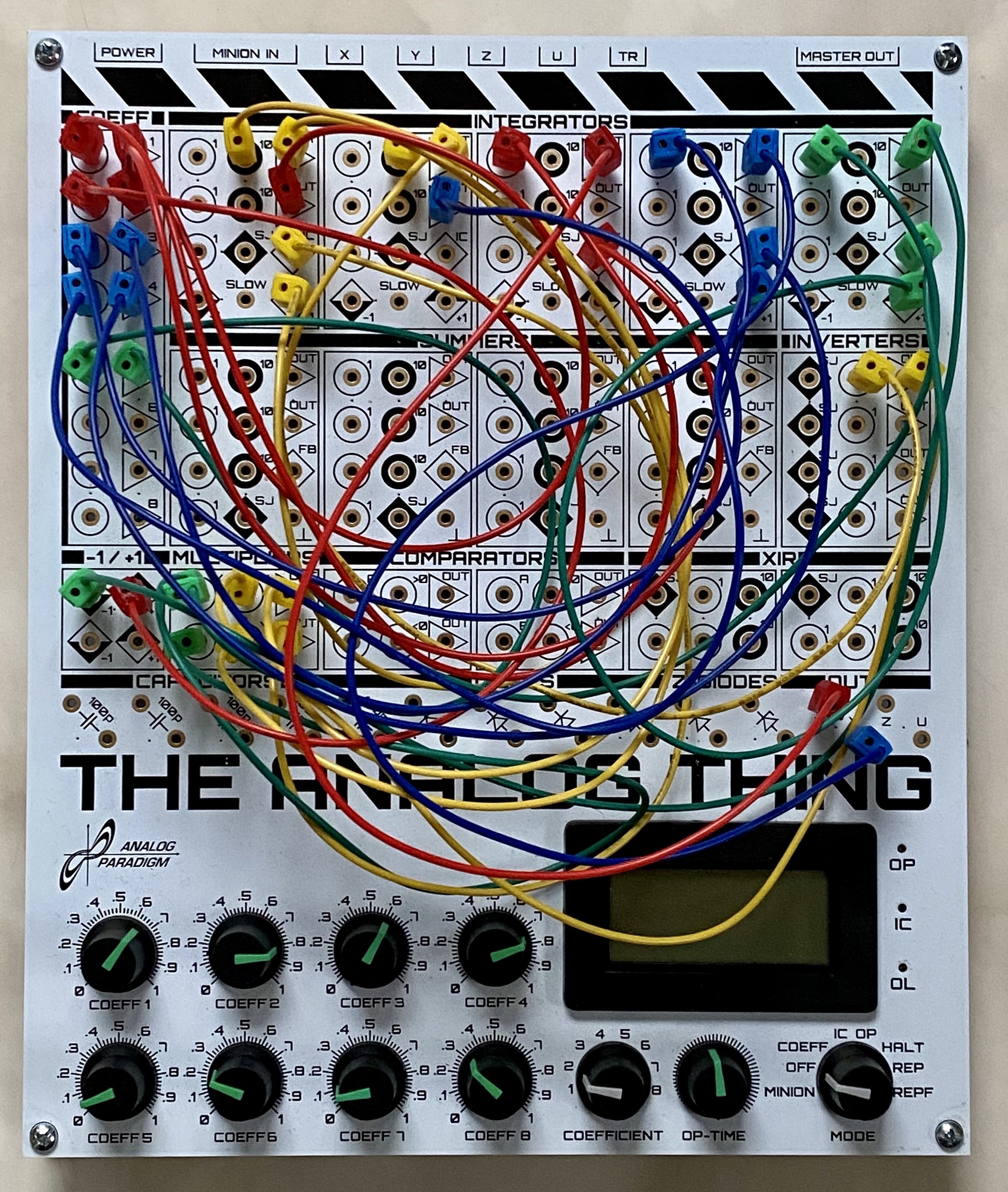
Figures 3 and 4 show the actual implementation of the program on THE ANALOG THING and a typical curve display as seen on an oscilloscope screen. The analog computer was set to repetitive operation and the operation time was set so that the output of the integrator yielding \(\dot{\varphi}\) is a ramp from \(-1\) to \(+1\) which corresponds to roughly \(20\) ms.
|

|
Figure 2: Setup for generating an Euler spiral Figure 3: Typical output of the Euler spiral pro- on THE ANALOG THING |
Figure 3: Typical output of the Euler spiral program |
Increasing the operating time slowly allows to show the growth of the Euler spiral on the oscilloscope screen. Ideally, all integrators are run with the highest time scale factor \(k_0\) selected. 2
References
[Havil(2019)] Julian Havil, Curves for the Mathematically Curious – an Anthology of the Unpredictable, Historical, Beautiful, and Romantic, Princeton University Press, 2019
[Ulmann(2020)] Bernd Ulmann, Analog and Hybrid Computer Programming, DeGruyter, 2020