Zombie Apocalypse Now
Introduction
How could one not like zombie movies? It was about time that someone, Robert Smith? and his collaborators, shed some light on zombie attacks from a mathematical point of view (see ). Phil Munz (see ) applied a well-known coupled set of differential equations to this particular problem, that was independently developed by Alfred James Lotka and Vito Volterra in the late 19th/early 20th century. Although Volterra and Lotka were interested in (closed) eco-systems, their equations are ideally suited to model a world infested by zombies. Whenever there is a problem which is readily described by (coupled) differential equations, an analog computer is the ideal tool to tackle them as we will do in the following.
Programming
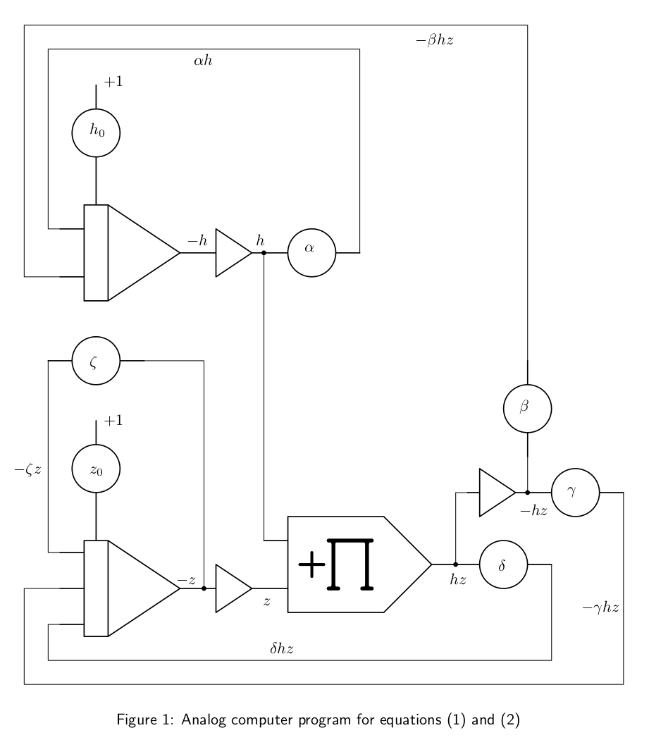
The mathematicsl model itself is quite straightforward and consists of the following two coupled differential equations:
\(h\) and \(z\) represent the number of humans and zombies, respectively. \(h_0\) and \(z_0\) are the initial conditions. The remaining parameters are
\(\alpha\): Growth rate of the human population (birthrate).
\(\beta\): Factor describing the rate at which humans are killed by zombies.
\(\delta\): Growth factor of zombie population due to zombies killing humans and thus transforming them into zombies.
\(\gamma\): Rate at which zombies are killed by humans.
\(\zeta\): Normal “death” rate of the zombie population.
Figure 1 shows the resulting program for the two equations while figure 2 shows the program as implemented on an Analog Paradigm Model-1 analog computer.
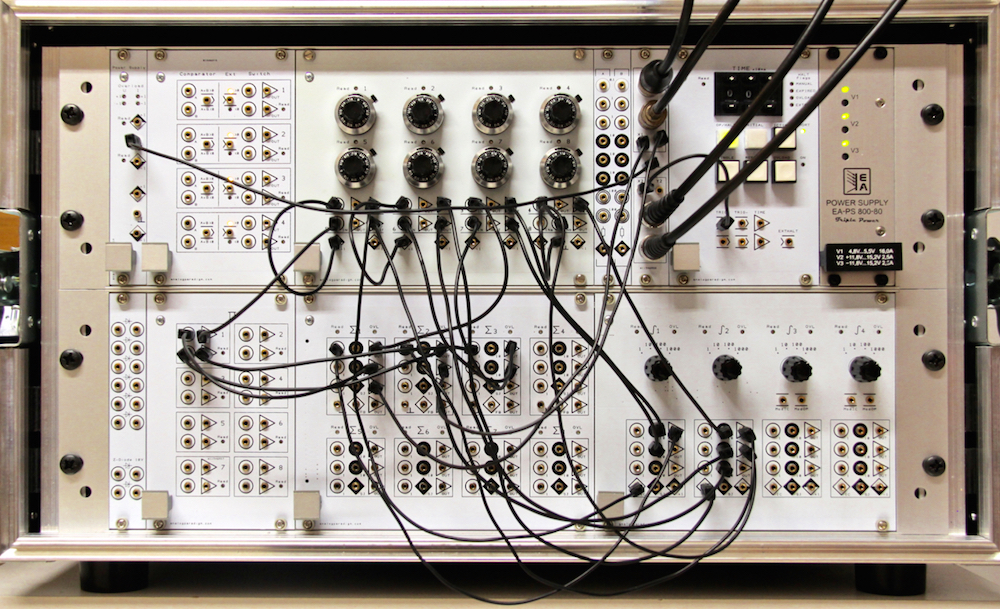
Zombie simulation on an Analog Paradigm Model-1 analog computer
Results
Figure 3 shows a typical result obtained with the setup described above. The computer was run in repetitive mode with the time-constants of the integrators set to \(k_0=10^3\). Additionally, only integrator inputs with a weight of \(10\) were used, further speeding up the simulation by another factor of \(10\). The IC-time was set to short, and the OP-time to \(60\) ms. The oscilloscope was explicitly triggered with one of the TRIG-outputs of the CU to obtain a stable, flicker-free display.
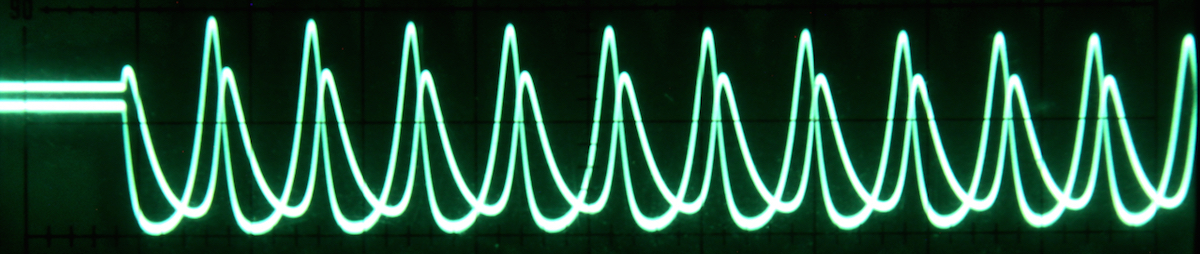
Results of a typical zombie simulation.
The parameters were derived experimentally by playing with the various coefficients until a stable behaviour was obtained. The output shown was generated with \(h_0=z_0=0.6\), \(\alpha=0.365\), \(\beta=0.95\), \(\delta=0.84\) (very successful zombies, indeed), \(\gamma=0.44\), and \(\zeta=0.09\).